
Akka Streams GraphDSL and Windowing
In a previous post we discussed about what it is windowing and how to implement it using Akka Streams. The main reason why we have to do this, and it is not provided by Akka Streams, it is because it’s a lower level library and let the developers manipulate the streams as they want. No boundaries, no limits.
As a continuation of the previous post, using the same codebase, we are going to explain the powerful GraphDSL provided by Akka Streams.
The input stream is based on sales records from a Kafka topic with the following format:
case class SalesRecord(transactionTimestamp: Long, shopId: Int, productId: Int, amount: Int, totalCost: Double)
The Kafka producer will be generating sales records that look like this:
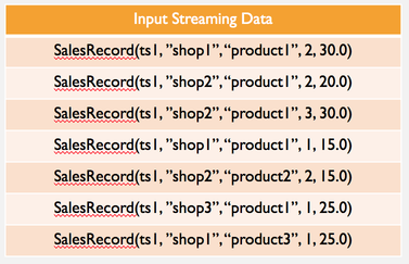
And we want to generate different aggregations to convert the incoming data into features that can be consumed by any machine learning library:
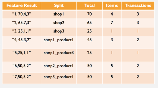
So this data seems to be something we could use to feed a ML algorithm.
In the following diagram we could have a nice overview about what we are going to implement:
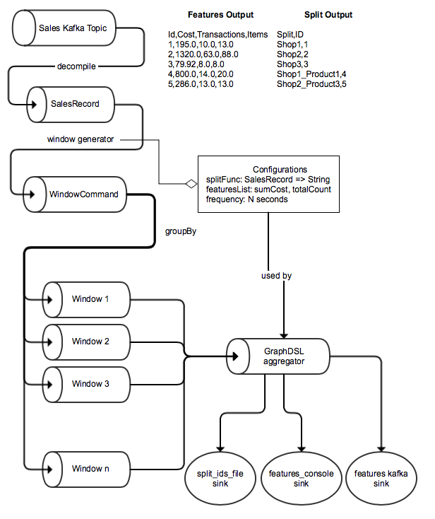
Let’s implement it.
Implementation
We have to model exactly this Graph using the Akka Streams GraphDSL:
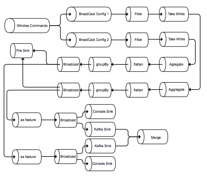
Apparently it could seem to be so complex, but the Akka Streams Graph DSL simplifies our work. As you can see the code start with one **Broadcast** operator and ended up in a **Merge** operator. Our graph will be a **FlowShape**, that means receiving one input stream and returning one output stream.
Before we enter into the GraphDSL implementation let’s summarize the implementation requirements:
- Define how to split the data
- Define how to create features
- Define the window frequency
This is the Config class:
  case class Config(id: Int, frequency: FiniteDuration, name: String, splitFunc: SalesRecord => String, featuresFunc: Seq[FeatureFunc], topic: String)
  case class FeatureFunc(name: String, func: Seq[SalesRecord] => Double)
As we can see, it contains a higher order function that converts a salesRecord to a String value. The featuresFunc contains a sequence of feature functions.
Here they are the config instances used in our example:
object Configs {
  import Domain._

  val totalCostFunc = (a: Seq[SalesRecord]) => a.foldLeft(0d)((agg, record) => agg + record.totalCost)
  val countTransactions = (a: Seq[SalesRecord]) => a.size.toDouble
  val countItems = (a: Seq[SalesRecord]) => a.foldLeft(0d)((agg, record) => agg + record.amount)

  val configs = Seq(
    Config(id = 1, frequency = 5 seconds, name = "shop", splitFunc = a => s"${a.shopId}",
      featuresFunc = Seq(
        FeatureFunc("sum", totalCostFunc),
        FeatureFunc("count_transactions", countTransactions),
        FeatureFunc("count_items", countItems)
      ), topic = "shop_features"),
    Config(id = 2, frequency = 12 seconds, name = "shop_product", splitFunc = a => s"${a.shopId}_${a.productId}",
      featuresFunc = Seq(
        FeatureFunc("sum", totalCostFunc),
        FeatureFunc("count_transactions", countTransactions),
        FeatureFunc("count_items", countItems)
      ), topic = "shop_product_features")

  )
}
Considerations about the previous code:
- Line 4: function that converts a sequence of sales records into a double value that contains the aggregation of all the record’s cost.
- Line 5: this one just counts the number of partitions.
- Line 6: this aggregation function stores the total of items per window.
- Line 9: contains the definition of the first configuration. It is splitting the data by shopId in 5 seconds windows. The output Kafka topic is shop_features.
- Line 15: contains the definition of the second configuration. It is splitting the data by shopId and productId in 12 seconds windows. The output Kafka topic is shop_product_features.
This Configurations will be used by our graph. The code to generate the graph is 70 lines long, so we are gonna explain portions of it:
  def createGraph() = GraphDSL.create() { implicit builder: GraphDSL.Builder[NotUsed] =>
    import GraphDSL.Implicits._
    val in = Inlet[WindowCommand]("Propagate.in")
    val bcast = builder.add(Broadcast[WindowCommand](configs.length))
    val merge = builder.add(Merge[ProducerRecord[Array[Byte], String]](configs.length))
    configs.map { config =>
      # Here we need to define all the different flows and sinks that define the graph


      bcast ~> filter ~> commands ~> aggregator ~> flatten ~> groupedBySplit ~> flattenMap ~> bcastListSalesGrouped

      bcastListSalesGrouped ~> slowSubFlow ~> fileSink
      bcastListSalesGrouped ~> toFeatures ~> bcastFeature
      bcastFeature ~> toProducerRecord ~> merge
      bcastFeature ~> printSink
    }
    FlowShape(bcast.in, merge.out)
  }
Considerations about the previous code:
- Line17: the function returns a FlowShape. A FlowShape is a flow object that contains exactly one input and one output.
- Line 3: This is the input of our graph. It is a stream of window commands.
- Line 4: Define a broadcast of WindowCommands. A BroadCast flow object, send the data from one input stream into N. In our case we will broadcast our input stream to 2 substreams, as we have 2 different split/window configurations.
- Line 6: we iterate over the our config files and then create all the different relationships in our graph.
- From the line 10 to the line 15 it is defined the Graph. As you can see, it directly correlates to the previous diagram showing what exactly has to do our Graph.
In the next fragment we are gonna see the first flows in the graph.:
      //Filter the windows that correspond to our frequency
      val filter = Flow[WindowCommand].filter(_.w.duration.get == config.frequency.toMillis)
      val commands = Flow[WindowCommand].takeWhile(!_.isInstanceOf[CloseWindow])
      val aggregator = Flow[WindowCommand].fold(List[SalesRecord]()) {
        case (agg, OpenWindow(window)) => agg
        case (agg, CloseWindow(_)) => agg
        case (agg, AddToWindow(ev, _)) => ev :: agg
      }
      val flatten = Flow[List[SalesRecord]].mapConcat(a => a)
Considerations about previous code:
- Line 2: it is an input of Window Commands that is filter out depending the config frequency.
- Line 3: important line here. Take records from the same window until you find out a CloseWindow command. This is the key of the windowing.
- Line 4: here it is done the aggregation suing the Flow fold operator. The output of this flow is a List of SalesRecords.
- Line 9: here the stream is flatten from a Stream[List[SalesRecord]] to a Stream[SalesRecord]. Good!
The next fragment of code shows the sinks definition and the features conversion:
      val groupedBySplit = Flow[SalesRecord].fold(Map[String, List[SalesRecord]]()) { (agg, record) =>
        val key = config.splitFunc(record)
        if (agg.contains(key)) {
          val current = agg(key)
          agg + (key -> (record :: current))
        } else {
          agg + (key -> List(record))
        }
      }
      val fileSink = Sink.foreach[(String, List[SalesRecord])](_ => SplitStore.saveToFile)
      val toFeatures = Flow[(String, List[SalesRecord])].map { entry =>
        val features = config.featuresFunc.map(featureFunc => featureFunc.func(entry._2)).foldLeft("")(_ + "," + _)
        s"${SplitStore.getId(entry._1)}$features"
      }
      val toProducerRecord = Flow[String].map { record =>
        new ProducerRecord[Array[Byte], String](config.topic, record)
      }
      val bcastFeature = builder.add(Broadcast[String](2))
      val printSink = Sink.foreach[String](r => logger.info(s"Producer Record: $r"))
Considerations about previous code:
- Line 1: using the flow fold operator to aggregate all the sales record that belong to the same split during the same window.
- Line 10: this line writes into the new feature ids into a file. The splits are formed by a concatenation of strings, but in our output dataset we need to convert the split attributes into one integer. This file will have the relationship between splits and ids.
- Line 11: we have as an input a map with String as key and a List[SalesRecord] as a value. In the definition of the Config we specified how it would be computed the features conversion using higher order functions.
- Line 12: here it is the computation of the features.
- Line 13: the output it is something like id, feature1,feature2,feature3…,feature_n
- Line 19: This is the definition of the console sink. Easy!
Source Code
I have not included all the source code during my explanations, but it is accesible from my github account: streams_repository
In case you want to run all the complete example, just follow the following instructions:
sbt docker
docker swarm init
docker stack deploy -c docker-compose.yml streams
docker service ls
docker logs -f $akka_producer_container
docker logs -f $spark_consumer_container
docker logs -f $akka_consumer_container
    http://localhost:8080 to access the spark cluster console.
docker stack rm streams
docker swarm leave --force
This will create:
- Kafka cluster
- Spark cluster
- Akka producer
- Akka consumer/producer using Graph DSL
- Spark consumer
Conclusion
Akka Streams is a very powerful tool to manipulate streams. It has some caveats, like for instance, it cannot execute into a cluster, but it could be a good solution in many cases.
I hope this example has not been tedious and you have fun. Any doubt you have about the code, do not hesitate to contact me.
And remember, the most important thing about my blog posts is that the code always work.